products for monitoring and diagnostics of machinery
A(M)Cademy of VIBROdiagnostics
#9 What is resampling?
Resampling, formally called “upsampling”, is a mathematical operation that converts a signal from the time domain to the angle domain. Resampling is performed mainly to reduce the negative impact of the machine’s changing rotational speed on the identification of the spectral components of the tested signal.
How does resampling work?
Let’s assume that we have a vibration signal in the form of a numerical series – classic “x” and a phase marker (PM) signal registered in parallel in the form of [0 … 0 0 1 0 0 ….. 0 0 1 0 … 0], where the value “1” means the next rotation of the reference shaft, as shown in Figure 1.

Figure 1. The idea of a phase marker (PM) signal in “once per revolution” mode
As a result of resampling, a “normal” signal, i.e. collected with a fixed number of samples per unit of time, e.g. 25 thousand samples per second, i.e. with a sampling frequency of 25 kHz, is converted into a signal with a fixed number (e.g. 20) of samples per revolution. Figure 2 and Figure 3 show what the resampling of the vibration signal with decreasing fundamental frequency looks like. This is a good example of the vibration of a machine in which rotational speed decreases.
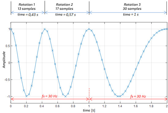
Figure 2. Signal with a fixed number of samples per unit of time
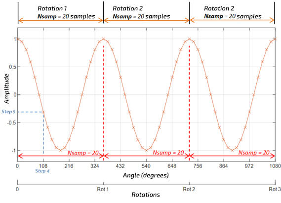
Figure 3. Signal with a fixed number of samples per revolution
Comparing Figure 2 with Figure 3, one can see that in the original signal, the first rotation is faster than the first rotation in the resampled signal, while in the case of the last, and third rotations, the opposite is true. This impression is correct because it follows that the higher the rotational speed of the shaft, the naturally fewer samples per revolution. In the output signal, the changes in velocity are not visible, and the rotation angle appears on the X-axis instead of time. The same number of samples are used for each rotation of the shaft.
The place of resampling in data analysis
Resampling is carried out in two ways, depending on the type of system in which we work:
DIAGNOSTICS system -> resampling performed on demand
MONITORING system -> automatic resampling
In the case of a diagnostic system, resampling is performed at the user’s (diagnostic expert) request, mainly to display the spectrum in the Order Spectrum (OS) domain, as shown in Figure 4.
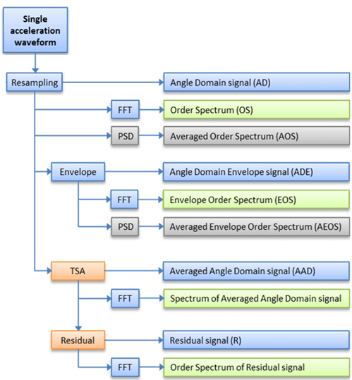
Figure 4. Resampling in the vibration monitoring system
In Figure 4, the names of 10 different types of figures often found in diagnostic analysis systems are presented, divided into individual signal processing stages that use resampling. The FFT block means calculating the spectrum in full resolution, while the PSD block (Power Spectrum Density) means the averaged spectrum (usually the signal power spectrum). The “Envelope” subgroup concerns the envelope spectrum (see post #7) of the resampled signal (Envelope Order Spectrum – EOS). The TSA block concerns Time-Synchronous Averaging, which is used to analyze vibration signals from drive systems with a relatively large number of gear ratios. In advanced systems, residual filtration (commonly known as Residual analysis) is also used to separate components of different classes of vibration signals.
In turn, in monitoring systems, resampling is an internal operation in the system, i.e. an operation invisible to the user. Figure 5 shows a general scheme in which the original vibration signal is first resampled and then transformed into one of the spectral forms (according to Figure 4). Then, based on the configured narrowband analyzes (see post #3), the system determines the spectral band (series indices), from which the final value of the trend point is calculated. Then, these values are compared with the alarm thresholds, which are the essence of the so-called events.
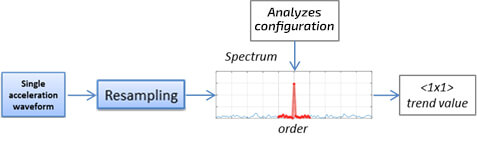
Figure 5. Resampling in the monitoring system (embedded system)
As one can see, resampling is a mathematical operation that does not play an autonomous role in the CMS system. Still, it is an indirect operation performed by a function or library, so further on we will discuss in detail the final functionality of this method from the point of view of the system user/diagnostic engineer.
What exactly does resampling do?
To answer this question, it is good to adopt the taxonomy from the previous section, because the presented division of architecture translates into functionality for the user. In the case of diagnostic systems, resampling enables easier identification of deterministic phase-locked spectral components (i.e. those whose frequency changes with the rotational speed of the machine). Resampling is therefore a method of signal processing, it enables the transition from the Hz domain to the order domain – at this point, let’s recall the appropriate figure from post #8.
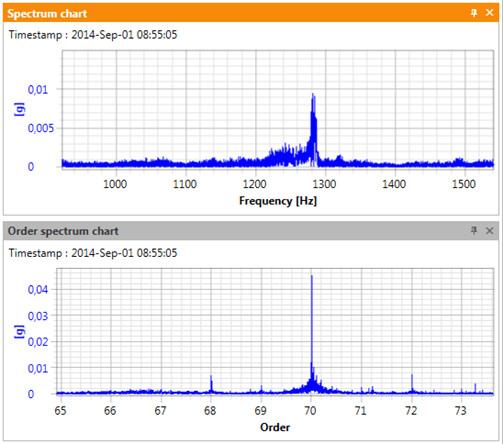
Figure 6. Comparison of the frequency spectrum and order spectrum
As shown in Figure 6, for a machine running at 1045-1100 RPM (see Figure 6 from post #8), the meshing component GMF = 70 order is in the range of 1219-1283 Hz, which makes it blurred and thus difficult to identify. While this component is somewhat visible on the frequency spectrum, the sidebands are only visible after resampling. On the other hand, on the order spectrum – which is the spectrum of the resampled signal (here in full resolution), even for such high frequencies and even for such large speed fluctuations, the meshing component is clearly visible, and with the pair of dominant sidebands (+/ – order*2).
Referring to the presented role of resampling in an autonomous monitoring system, one should notice that in the case of the analyzed overlapping component, its trend is related to the designated spectral band and works differently in the case of two types of spectra. Figure 7 will help us clarify 2 main problems. First of all, let us note that in the frequency domain (Figure 7 – top) the position of the band depends on the rotational speed, so each time the speed changes, it must be recalculated. In addition, the limit values of the band marked in Figure 7 (top) were determined a posteriori based on the range of rotational speed variability. It is clear that it would be difficult to establish consistent limit values without these data. On the other hand, in the case of the order spectrum, a band was marked which centre is always in the same place (70th order), and which width can be easily set – typically as 3% of the middle band value (in Figure 7 – bottom, for easy visualization, a bandwidth of +/-2.8% was assumed).
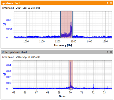
Figure 7. Definition of spectral bands for frequency spectrum and order spectrum
The discussed analyses concern the tracking of the power (rarely RMS or energy) of the signal in bands that include several dozen, and sometimes several hundred spectral points. However, when single peaks from the bands (maximum values of the amplitude) are tracked, the importance of resampling is even greater, because fuzzy spectra are not suitable for determining such components.
Synchronous averaging
The resampled signal can then be averaged over the shaft revolutions, which significantly improves the signal (in the case of deterministic synchronous components) to noise ratio. Such an analysis is called a “synchronously averaged” analysis. In English it is a bit worse, historically called TSA, for Time-Synchronous Averaging, although the averaging is done in the angular rather than the time domain. Figure 8 shows, from top to bottom: a fragment of the original vibration signal per one revolution of the shaft, a fragment of the resampled vibration signal per one revolution of the shaft and the average signal TSA, which contains only one revolution of the shaft. In addition, in the middle and bottom graphs, the signal resampled with respect to the Fast Shaft (FS) is marked in blue, and the signal resampled with respect to the Slow Shaft (SS) is marked in red. On the TSA signals, we see 23 cycles for the fast shaft, and 67 cycles for the slow shaft, during one revolution, because the shafts are connected by a single-stage gear with gears with 23 and 67 teeth, respectively.
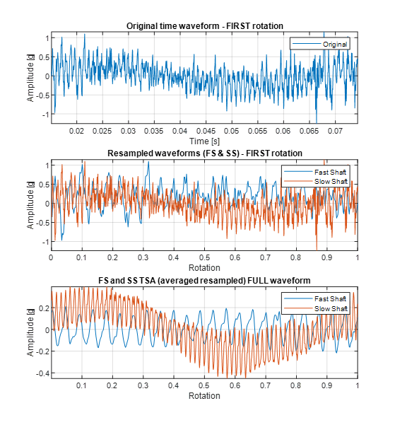
Figure 8. Definition of spectral bands for frequency spectrum and order spectrum
Analyzing Figure 8, one may notice that:
- the TSA signal for the free shaft is significantly denoised both in relation to the original signal and the resampled signal,
- the TSA signal for the fast shaft is significantly denoised in relation to both the original signal and the resampled signal,
- TSA signals show that the cooperation of successive pairs of gear teeth generates a slightly different vibration component each time.
In addition, it is worth mentioning that the general shape of the original signal coincides with the general shape of the free shaft signal, so in the case of the fast shaft, the resampled signal and TSA are stretched (containing fewer points in one revolution). The presented synchronous analysis is quite difficult to implement, but it is extremely valuable when analyzing drive systems with a large number of shafts because it allows obtaining much cleaner signals for the analysis of vibrations in subsequent gears.
The long-awaited math for the avid reader
When working with spectra, it is good to know the basic principles of their parameterization. The starting point is always the original signal of length T seconds recorded with the sampling frequency fs. Let us remember that the full spectral resolution is the reciprocal of the signal duration (1/T) and the spectral range is half the sampling frequency (fs/2). Table 1 shows how the quoted relationships translate into the angle domain and the order domain for the resampled signal. Table 2 illustrates a numerical example for Table 1.
Table 1 – Parameters of a resampled signal and its spectrum in full resolution
| Parameter | Time domain | Order domain |
| Signal Length | T [s] | Nrot (quantity) |
| Sampling | fs (frequency) | Nsamp (number of samples per revolution) |
| Resolution (time/angle) | dt = 1/fs | d_rot = 1/Nsamp |
| Spectral resolution | df = 1/T (also fs/number of samples) | d_ord = 1/Nrot |
| Spectral range | fs/2 | Nsamp/2 |
| X-axis (time/angle) | dt:dt:T | d_rot:d_rot:Nrot |
| X-axis (spectrum) | 0:df:fs/2 | 0:d_ord:Nsamp/2 |
Table 2 – Parameters of a resampled signal and its spectrum in full resolution
| Parameter | Time domain | Order domain |
| Average speed 2000 RPM | – | – |
| Signal Length | 10 [s] | Nrot = 333,3 |
| Sampling | 25 kHz | Nsamp = 1500 |
| Resolution (time/angle) | dt = 0,00004 [s] | d_rot = 0,00066 |
| Spectral resolution | df = 0,1 Hz | d_ord = 0,003 [ord] |
| Spectral range | 12,5 kHz | 750 [ord] |
| X-axis (time/angle) | 4e-5:4e-5:10 | d_rot:d_rot:Nrot |
| X-axis (spectrum) | 0:0,1:12500 | 0:0,003:750 |
For a shaft revolving with the speed of 2000 RPM, the number of revolutions in 10 s is:
Nrot = Speed/60*T = 2000/60*10 = 333,3 revolutions
Let’s set the new number of samples per revolution as twice the average of the number of samples per revolution. Of course, we do not have data describing individual revolutions, so let’s use the general mean relationship:
the average number of samples per revolution N_avg = number of samples per second fs/number of revolutions per second (speed [Hz])
N_avg = fs / (Speed in Hz) = 25000/(2000/60) = 25000/ 33.3 = 750
Nsamp = 2*N_avg = 2*750 = 1500
The remaining values result directly from substitution to the formulas from Table 1. In practical applications, it is additionally ensured that both the number of samples per revolution and the number of revolutions are even, and the signal is trimmed to full revolutions, as this has a positive effect on the length of the calculations. Let’s add that the TSA signal is calculated by averaging the given signal resampled over subsequent shaft revolutions (i.e. a signal that recorded 500 revolutions of the shaft will be the result of 500-fold averaging). Therefore, for TSA signals, the number of points per revolution Nsamp is the same as for the resampled signal, while the number of revolutions Nrot is equal to 1.
Resampling myths
It is interesting to note that the new number of samples per revolution Nsamp, determined in step 3 of the general algorithm (see section “WHAT IS RESAMPLING”), historically was usually equal to the power of 2 closest to the average number of samples per revolution in the original signal. This is related to the speed of the FFT calculation algorithms (in the process of further determination of the order spectrum). However, from the analytical side, the new number of samples per revolution:
- should be greater than the largest number of samples per revolution present in the signal (otherwise the unfavourable phenomenon of aliasing will be present),
- it is the better, the greater the multiple of the average number of samples per revolution in the original signal (due to the reduction of the power of the sidelobes, generated during the convolution of the signals as part of the resampling calculation).
Similarly, higher-order interpolation functions (especially chip and spline) generate sidelobes with lower power – i.e. a less noisy (“better”) signal. However, from a practical point of view, the use of advanced computational techniques is often of little importance in assessing the technical condition of the machine, and additionally significantly extends the calculation time. For this reason, industrial systems often “bend” the math a little at the expense of relatively small losses in the quality of the signals being analyzed. Specifically, often the new number of samples per revolution Nsamp is equal to the nearest number from the predefined set, for which the given processor calculates the FFT as quickly as possible (these do not have to be powers of 2 because there are also numbers for which calculations take an extremely long time). In addition, within the framework of two-step interpolation, simplified linear interpolation is often used, based on solving a system of 2 equations with 2 unknowns of the form y = ax + b, which is a somewhat primitive but effective solution.
Let’s add that resampling “improves” only the position of the components on the spectral axis, and the change in their amplitude (visible as a beneficial increase in the amplitude of the observed components) is only a consequence of this operation. Unfortunately, we sometimes forget about it and use resampling to analyze signals that were registered with significant changes in rotational speed. This approach is risky because it introduces an error in the amplitude assessment – with a large change in operating parameters, not only does the excitation value change but also the modal parameters of the machine change (in a way practically unknown to us) and thus its frequency response function changes, which can have a very large impact on the change in the amplitude of the components after resampling – a change that does not result from resampling. Therefore, just like in post #8, we recommend that resampling be allowed in practical technical diagnostics only in cases where the maximum rotational speed deviations in the processed waveform do not exceed a few per cent.
Use of measuring equipment
AMC VIBRO offers systems that allow for both automatic resampling and resampling on demand. Depending on the product version, the systems calculate the order-domain spectrum and the order-domain envelope spectrum, as well as narrowband analyses, including analyses of TSA signals.
Table 3 Juxtaposition of AVM family devices in terms of resampling
| AVM 2000 | AVM 4000 | |
| Synchronous analysis | ✔️ (selected models) | ✔️ |
| Resampling on demand (max. 300 [s] with fs = 25 kHz) | ✔️ | |
| Definition of narrowband analyses in order domain (OS spectrum), (selected models) | ✔️ (selected models) | ✔️ |
| Definition of narrowband analyses in order domain (EOS spectrum) | ✔️ | |
| Definition of TSA analyses | ✔️ |
Book recommendation