products for monitoring and diagnostics of machinery
A(M)Cademy of VIBROdiagnostics
#3 What is characteristic frequency?
Before we proceed to explain the term “characteristic frequency” one needs to explain a delicate difference between several similar concepts:
- Signal component – a signal component in time domain (mainly sine wave or noise),
- Spectral component – a spectral “stripe” or something different on the spectrum that can be seen, measured and described
- Frequency component – a spectral “stripe” which frequency can be read,
- Characteristic component – a component of a signal which can be referred to a machine element,
- Characteristic frequency – a spectral “stripe” which can be referred to a machine element (the name is also typically used – incorrectly – in order domain).
In the best-case scenario of machine diagnostics, each mechanical element of a rotor machine generates a unique set of vibration signal components. Picture 1 symbolically depicts exemplary sets of such characteristic components, generated respectively by a toothed gear, drive shaft and rolling bearing.
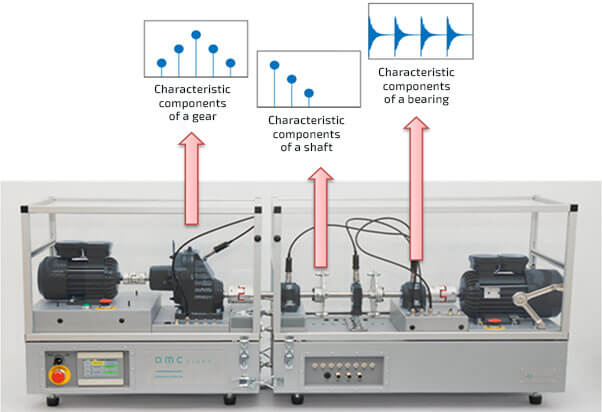
Picture 1 Characteristic components of a gear (frequency domain), shaft (frequency domain) and bearing (time domain)
Picture 1 shows two frequently found types of characteristic components in the frequency domain (that is frequency components) – gear sidebands and harmonic components for a shaft and one type of characteristic components in the time domain – impulse responses for a bearing.
In each case, all signal components are first represented as the original vibration signal in the time domain (more rarely in the degree domain) later, however, process paths may differ.
For example, characteristic components of the bearing shown in the time domain in Picture 1 are the result of calculating the envelope of the signal which can be made in the frequency domain. As a result, if the given spectral component is analyzed on the envelope spectrum (and not the “normal” spectrum of the original signal) this fact should always be noted because the same characteristic component in different kinds of spectra may indicate various forces acting on a machine, therefore comes down to a different diagnostic conclusion.
So then, where do the concepts of spectral component and characteristic frequency converge?
Knowledge of “characteristic frequency” enables partial assignment of spectral components to specific elements of a machine, therefore it is connected with the issue of identifying machine damages.
Although it is not entirely obvious, characteristic components are a concept that precedes the concept of characteristic frequency, additionally, they generally refer to the degree spectrum of the presented signal, therefore to the order spectrum, which will be explained step-by-step. In other words, those two simple terms are connected with one slightly more difficult concept. Table 1 shows a set of exemplary spectral components related to the respective parts of a rotor machine.
Table 1 Exemplary characteristic frequencies.
| Machine element | Type of plot | Spectral component | Type of damage |
| Drive shaft | spectrum | 1x | unbalance |
| Drive shaft | spectrum | 1x, 2x | misalignment |
| Drive shaft | spectrum | 1x, 2x, 3x | foundation backlash |
| Fan blades | spectrum | RPM*number of blades | damaged blade |
| Toothed gear | spectrum | GMFx1, GMFx2 | local damage |
| Toothed gear | spectrum | DSBx1, DSBx2 | change of geometric dimensions |
| Rolling bearing | envelope spectrum | BPFO 1x, 2x, 3x | local damage to the outer ring |
Indications:
RPM – rotational speed,
GMF – frequency of gear meshing (number of teeth on a wheel on a given shaft*RPM)
DSB – sidebands (left and right)
BPFO – frequency (of damage) of the outer ring of a rolling bearing
One needs to remember that in practical use the presence of a component does not necessarily indicate machine damage. For example, a series of shaft harmonics is typical for “healthy” piston compressors. Moreover, a lot depends on construction – in the case of straight-toothed gear, damage usually manifests as an increase of GMF components, yet in the case of spiral gear, it manifests as an increase of sidebands of GMF components. However, one can say that detection and observation of an increase of characteristic frequency energy are the most effective and the most frequently used method of detecting damages to rotor machines.
As mentioned earlier, in tables such as Table 1 one generally gives characteristic orders and within practical analysis describes characteristic frequency. The description of the transition will be shown below, along with an example.
The idea of “characteristic orders”
Let’s discuss a frequency component illustrating an unbalance of a free shaft mounted on an AV TEST BENCH stand, shown in Picture 2.
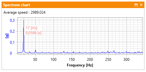
Picture 2 Unbalance on the frequency spectrum
If the free shaft of the machine rotates with a nominal speed of 1000 rotations/minute (1000 RPM), its “characteristic frequency” equals:
f_char = 1000/60 = 16.7 Hz
which approximately (for spectral resolution of 1 Hz) gives 17 Hz. On the order spectrum, the characteristic order of the shaft is related to its gear ratio with respect to the measurement of the rotational speed of the fast shaft. The gear ration on the AV TEST BENCH stand equals 23/67 = 0.343. The characteristic component illustrating the free shaft unbalance on the order spectrum is shown in Picture 3. For example, if the main high-speed shaft was unbalanced, “Order =1” in picture 3 would be replaced with a different characteristic component.
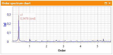
Picture 3 Unbalance on the order spectrum
Aside from the computational issue mentioned before, there are 2 other crucial reasons why order spectra are used in the practical analysis, which will be mentioned below:
1) Due to rotational speed fluctuation in real-valued signals, frequency components tend to be fuzzy. It is worth noting that the higher the frequency of a deterministic (of singular frequency) component the fuzzier it becomes. Because of that, in rotor machines diagnostics “characteristic orders” are often analyzed instead of characteristic frequency. For example, Picture 2 depicts a typical frequency spectrum for a drive shaft unbalance. For comparison, Picture 3 shows the same state on the order spectrum.
2) Besides lesser fuzziness of components (especially in higher frequency) the most important merit of order analysis (with respect to frequency analysis) is the fact that along with the change in rotational speed, components do not change their position on the spectrum.
With a basic understanding of order analysis, we can return to characteristic frequencies. For those interested – we will come back to order analysis later.
Analysis example
As an example of characteristic frequency analysis let us consider characteristic components of the toothed gear on AV TEST BENCH stand. Data provided by the producer:
Z1 = 23; number of teeth of the small gear (fast shaft – INPUT Shaft),
Z2 = 67; number of teeth of the large gear (slow shaft – OUTPUT Shaft).
In first step we build a kinetostatic pattern in Kinematic Editor in VIBnavigator environment. The finished scheme is shown in Picture 4.
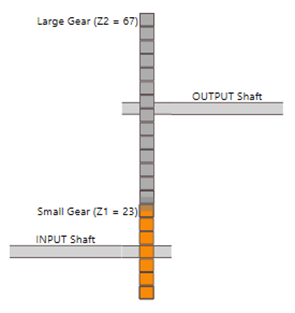
Picture 4 Toothed gear diagram
Having marked the reference shaft (INPUT Shaft), in the second step Kinematic Editor automatically calculates order characteristics for several subsequent Gear Meshing Frequency GMF, and then calculates order characteristics for several consecutive pairs of double sidebands – DSB. Table 2 shows 4 GMF values and 2 pairs of sidebands from the fast and slow shaft for the first GMF.
Table 1 Exemplary characteristic orders
| GMF harmonics | order |
| Przekładnia.GMFx1 | 23,00 |
| Przekładnia.GMFx2 | 46,00 |
| Przekładnia.GMFx3 | 69,00 |
| Przekładnia.GMFx4 | 92,00 |
| GMF sidebands | order |
| Przekładnia.GMFx1+Gear1x1 | 24,00 |
| Przekładnia.GMFx1+Gear1x2 | 25,00 |
| Przekładnia.GMFx1+Gear2x1 | 23,34 |
| Przekładnia.GMFx1+Gear2x2 | 23,69 |
| Przekładnia.GMFx1-Gear1x1 | 22,00 |
| Przekładnia.GMFx1-Gear1x2 | 21,00 |
| Przekładnia.GMFx1-Gear2x1 | 22,66 |
| Przekładnia.GMFx1-Gear2x2 | 22,31 |
In order to illustrate it, Picture 5 depicts an exemplary order spectrum on which one marked characteristic gear meshing frequency (more accurately: characteristic order) on the AV TEST BENCH GMFx1 alongside the pair of fast shaft sidebands (order 1, so 23 +/-1) as well as two right and one left sideband of the slow shaft (order 0.343, so Right: 23+0.343*1, 23+0.343*2 and Left: 23-0.343*1).
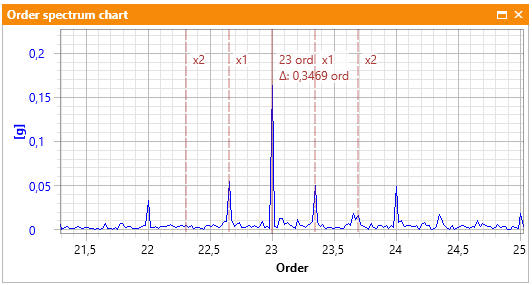
Picture 5 Spectral component GMFx1i and its sidebands.
As mentioned before, in engineering practice we often reference “frequency” terms when analyzing order data – the component name itself GMF “Gear Meshing Frequency” partially justifies it.
Third, a very important engineering step is (always slightly subjective) defining the mathematical relation between an “ideal” characteristic order and an order band. In practice, the point is to “give a certain width to every stripe defined” on the spectrum, which will be monitored by the diagnostic system. The value of around 3% is often used here. For example, after using that method, a “nice” number 23 is replaced with two “ugly numbers”:
Bin_start = 23 + 3%*23 = 23,69(order)
Bin_stop = 23-3%*23 = 22,31(order)
Usually, however, the operation is invisible to monitoring system users.
In the last step characteristic orders, bin_start and bin_stop are changed to final characteristic frequencies according to the formula:
f_char_start = bin_start*average machine speed [Hz]
f_char_stop = bin_stop*average machine speed [Hz]
Obviously within preparing the diagnostic analysis, “ideal” characteristic orders are often converted to “ideal” characteristic frequencies using average machine speed, e.g. average_velocity = 1000Hz GMF = 23(order) f_char_GMF = 23*1000/60 Hz = 383.3 Hz
Thanks to that we know the component within a close range from 383 Hz is probably related to the gear meshing.
What do characteristic components help us with?
A lot actually! In diagnostic practice, characteristic components are used in two main ways. If discussing a large monitoring system, the definition of characteristic order/frequency is the primary system configuration within the narrowband analysis. The accurately defined narrowband analysis described with the name of a mechanical element is the key to effective monitoring of the technical condition of an object, ideologically shown in Picture 6.
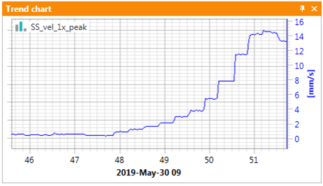
Picture 6. Rapid growth of pump rotor unbalance
When talking about data analysis (technical diagnostic), characteristic orders/frequencies help us identify spectral components – which is what we actually started this post with! An identification example can be found in Picture 5.
The use of measuring devices
AMC VIBRO company offers both the way of measuring characteristic components defined by the user and characteristic components automatically calculated by the system according to the kinetostatic model.
Table 2. The Juxtaposition of AVM family devices in terms of characteristic frequency
|
|
|
|
|
| Tracking user’s characteristic components in the frequency domain | ✔️ | ✔️ | |
| Tracking user’s characteristic components in order of domain | ✔️ | ✔️ | |
| Automatic calculation of characteristic orders of machine elements | ✔️ | ||
| Automatic calculation of characteristic frequencies of machine elements | ✔️ |
Book recommendation