products for monitoring and diagnostics of machinery
A(M)Cademy of VIBROdiagnostics
#8 What are variable operating conditions?
From the point of view of practical vibrodiagnostic analysis, rotating machines can be divided into two groups – devices operating in constant operating conditions and machines operating in variable operating conditions.
Operating conditions, also known as “operating parameters” or “operating points” of a machine, are a set of various parameters that describe how the machine works at a given moment. The most common operating parameters for virtually all rotating machinery are rotational speed, power/load and temperature. The list of key operating parameters for many machines can be much longer.
An example of vibrations from a machine operating in variable operating conditions is shown in Figure 1. As one can see, within five minutes the vibration level changed significantly – even by 100% – but it did not result from a change in the machine’s technical condition, but from changing the operating point. Thus, diagnosing machines operating under changing operating conditions is a great challenge. Not every monitoring system can handle it.
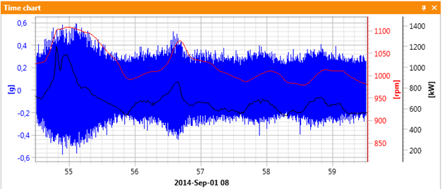
Figure 1 Vibration signal of a machine working in variable operating conditions
Why do operating conditions matter?
To answer this question coherently, we will first briefly cover two introductory topics:
1. Registered vibration signal
As part of typical technical diagnostics, we use an accelerometer to measure vibrations of the housing of a machine element. This signal is defined as the “response” of the system to input forces. A simple case may be a rotor machine in which the shaft is driven by electromotive force. As Fig. 2 shows, the resulting spectrum of the signal, which we record, for example, on the bearing housing, is much more complicated than the Shaftx1 component (although it typically includes the Shaftx1 input component), because – to put it simply – it depends on the nonlinearity of the system and the so-called frequency response function of the system (FRF – Frequency Response Function). Let’s leave FRF for a moment and move on to the first conclusion.
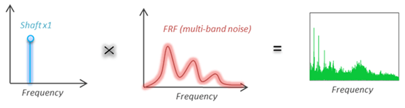
Figure 2 The idea of measuring the vibration of a rotor machine
CONCLUSION 1: If we make two measurements of our machine vibration and get two significantly different signals, it may be caused either by a change in the input forces or a change in FRF or – which tends to cause the most trouble – simultaneous change in forces acting on the machine and change in FRF.
2. Modal analysis
Whether the reader likes it or not, every real object, and thus every rotating machine, is subject to the laws of physics. Therefore, modal analysis is applied to it, which deals with e.g. determining the FRF shown in Figure 2. Many books can be written (and read) about modal analysis, but in this post, we will only present four observations that are necessary to gain some intuition:
- The modal analysis will answer the question, of why the washing machine vibrates the most when reaching full rotational speed, and not after reaching it
- The modal analysis determines the frequency of bell ringer work so that the heart of the bell works „opposite” to its shell
- The modal analysis is capable of explaining, why stiffening the foundations changes the vibration signal recorded by the accelerometer from the bearing housing
- The modal analysis explains why measuring vibrations in a different direction or using a different sensor pad can give significantly different signals
Moving on to the diagnostician’s dictionary, thanks to Modal Analysis, each object can be characterized in a simplified way as a set of eigenfrequencies, each of which is described by mass, damping coefficient and elasticity coefficient. Importantly, classic Modal Analysis assumes that we study stationary objects (parameters do not change over time) and linear objects (parameters do not depend on the operating point), which is a significant simplification. At this point, we turn to the second conclusion.
CONCLUSION 2: It is easy to imagine that when a machine experiences a change in load (or other operational parameters), its stiffness and elasticity parameters change, and so its FRF changes as well, leading to a change in the vibration signal we are analyzing.
Now, combining both conclusions, we can assume, that:
- a change in the rotational speed of the machine must change the spectral distribution of the recorded signal because the frequency of the forces acting on subsequent elements of the drive system changes (see component Shaftx1),
- depending on the current “shape” of the FRF of the machine, the change in the spectral distribution of the recorded signal may be very different, because the change in the rotational speed of the machine may take place in the “safer” ranges (e.g. FRF relatively flat in the vicinity of Shaftx1)
- little effect on the spectrum or may cause a dangerous increase in vibration (here the reader is referred to the section ” modification of the 1x component by critical velocity” in post #4
- great influence on the spectrum
- changing the load or correlated parameters must change the spectral distribution of the recorded signal because the modal parameters (stiffness and damping) change.
In the practical analysis of vibration signals, however, we will quickly see that this is not the end of the story. We often observe the mutual correlation of speed and load, e.g. for asynchronous squirrel-cage motors. For example, it is easy to see that an increase in load typically results in a noticeable decrease in rotational speed. Similarly, the other way around – as the speed increases, we provide additional energy to the vibration signal, which will be visible to us as an “increase” in the amplitudes of structural frequencies on the spectrum.
An Exemplary machine
It is quite easy to imagine that the vibration of the machine increases alongside its speed. This is in line with our intuition. But it is more difficult to justify why vibrations decrease with increasing rotational speed, and such situations also happen. In figure 3, we present a rather rare graph – a surface illustrating the effective value of vibrations (RMS) of the machine depending on the quite densely measured rotational speed and load. As can be seen in figure 3, there is a certain global trend of vibration increase with the increase of both operating parameters, but it is quite easy to notice significant local minima and local maxima – related to both the critical speed and the changes in the FRF of the system.
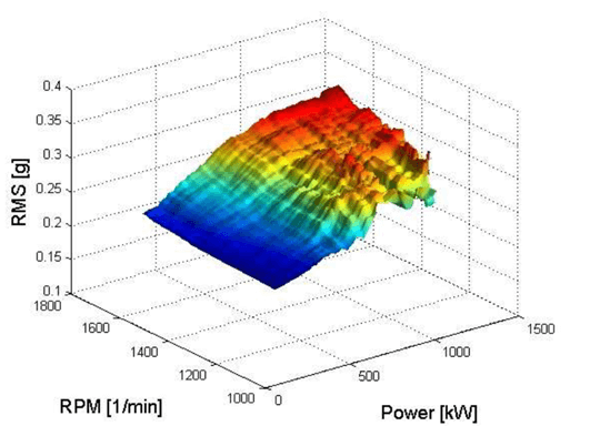
Figure 3 Impact of rotational speed and load changes on the level of vibrations
For example, for a power of 1000kW, in the range from 1600 RPM to 1800 RPM, we will observe a monotonic increase in vibration with the increase in rotational speed, however in the range from 1400 RPM to 1600 RPM we can expect a decrease in vibration.
Methods of analyzing machines operating in variable operating conditions
When our task is to assess the technical condition of machines operating in changing operating conditions, we have a choice of several proven tools and several new concepts.
Defining operating states
Firstly, some monitoring systems (including the AVM 4000) allow several operating states to be defined for each machine. These may be, for example, the following states: “nominal power”, “low speed”, “turbine operation”, “pump operation”, etc., depending on the type of machine and the way it is used. During configuration, the user indicates what values the operational state depends on and what it is called. More advanced systems allow operating states to be dependent on more than one parameter.
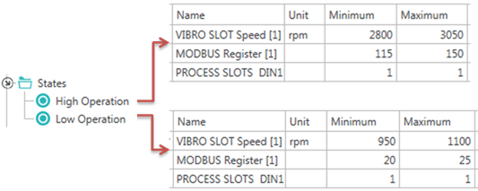
Figure 4 Exemplary definition of High state and Low state
When working, the monitoring system automatically recognizes the operational state of the machine. Different levels of alarm thresholds and different data recording rules can be defined for each state, as shown in figure 4.
The ability to define operating states is a very powerful tool for dealing with changing operating conditions. On the other hand, remember not to define too many of them, because then you need to define alarm threshold values for each of them … As always, it is worth using common sense.
Selective choice of data
An even more effective way to use Operational States is not only tracking operating parameters during the acquisition but also selecting the “best” waveforms. This is important because data – especially raw vibration data – takes up a lot of space, and for analysis, we do not need a lot of data, only data reflecting the state of the machine. Figure 5 illustrates the idea of selective registration implemented by the AVM 4000 system by AMC VIBRO.
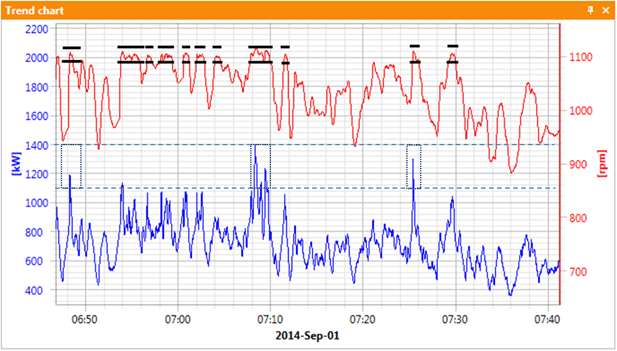
Figure 5 The idea of selective registration
In the given example, the definition of the “High” state is shown, i.e. rotational speed of 1975 RPM-2050 RPM and power in the range of 1100 kW-1400 kW. For such defined values, the AVM 4000 system automatically determines when the logical conjunction takes place and then registers the set number of waveforms in the interval (e.g. 1 waveform per day). Figure 5 shows that the conjunction is met in three-time intervals. The result of such functionality is the ability to monitor machines operating even in highly variable operating conditions as if they were working in stationary conditions. The disadvantage of this solution is asynchronous data recording (i.e. we do not have a fixed number of trend points in a given time interval).
Resampling
Thirdly, we can try to measure and compensate for the impact of changing operating conditions. It’s relatively simplest to do it for a variable rotational speed. In this case, it is worth using the resampling technique, which makes the position of the characteristic spectral components independent of the rotational speed and presents the spectrum in the domain of orders, not frequency (see Post #2, section “The idea of characteristic orders”). Figure 6 shows an exemplary vibration signal and the instantaneous rotational speed.
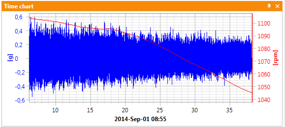
Figure 6 Vibration signal with a slight change in rotational speed
As can be seen in Figure 6, a change in the rotational speed at the level of 5% significantly affects the level of the signal amplitude. In practical technical diagnostics, it is recommended that the change does not exceed 2%. Figure 7 shows an exemplary spectrum in Hertz and its transformation in the domain of orders from the same vibration signal, calculated in the VIBnavigator program by AMC VIBRO.
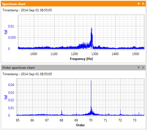
Figure 7 Comparison of the frequency spectrum and order spectrum
As seen in Figure 7, the analysis of components in the order domain is simpler because the spectrum is not fuzzy.
Definition of narrowband analysis width
When we are interested in monitoring, i.e. trend analysis, for machines operating in variable operating conditions, it is worth defining not specific frequency/order values, but bands. For example, as shown in figure 8, the “Kinematics Editor” module of the VIBnavigator environment allows you to define the bandwidth for each type of machine element separately, e.g.:
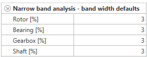
Figure 8 Definition of the band adaptation to the spectral blur level
It is worth noting that resampling never works “perfectly”, and the blurring error increases proportionally to the frequency/order of the component, so it is worth using this option even for components defined in the order domain.
Automatic data validation
An additional advantage of the AVM 4000 system is the automatic data validation module, which is particularly important in the process of diagnosing machines operating in extremely variable operating conditions, such as wind turbines or mining machines. The True Data Validator™ module implemented in the embedded system ensures that the system will not process data registered incorrectly (or containing unwanted “shots”), which significantly reduces the number of false alarms FAR (False Alarm Rate).
Application of measuring equipment
AMC VIBRO offers systems that allow for automatic resampling, the variable definition of bandwidths, data registration based on the definition of user states and automatic data validation.
Table 1 Juxtaposition of devices of the AVM family in terms of diagnostics of machines operating in variable operating conditions
|
|
|
|
| Automatic resampling | ✔️ (selected models) | ✔️ |
| Definition of the width of broadband analysis in the frequency domain | ✔️ | ✔️ |
| Definition of the width of broadband analysis in the order domain | ✔️ (selected models) | ✔️ |
| Definition of the width of narrowband analysis in the frequency domain | ✔️ | ✔️ |
| Definition of the width of narrowband analysis in the order domain | ✔️ (selected models) | ✔️ |
| Ability to define operating states | ✔️ | |
| Selective data selection module | ✔️ | |
| Automatic Data Validation Module | ✔️ |


Book recommendation