A(M)Cademy of VIBROdiagnostics

#7 Why is early detection of rolling bearing damage so important?

01.02.2023

Rolling bearing damage is one of the most important causes of rotating machine deterioration. However, early detection allows for a relatively cheap replacement. If the relevance degrades, there are negative consequences, worn products get into the oil, and the work of the shaft changes, which in turn begins to destroy following machine components, e.g. gears, clutch and other bearings. In extreme cases, the destruction of bearings leads to various types of disasters, e.g. plane crashes ^[1].

Signal envelope analysis

In the early stage of damage development, the rolling bearing excites its structure and housing according to the so-called “characteristic damage frequency”. Let’s assume it’s a frequency, say 90 Hz. You can imagine that this is a situation where the machine is not running and some small hammer hits the cover 90 times a second. Next, we take a measurement that lasts 1 second. What will such a signal look like? – We will see the fading impulse responses, as shown in Figure 1.

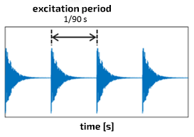
Figure 1. Fading impulse responses

The development of science (Fourier analysis and modal analysis) has made it possible for us to read and interpret the frequency composition of such a signal sequentially, both for a single impulse response and for many responses at once. Thus, in the case of typical bearing housings, the frequency composition of such a signal looks like various types of “hills” in the band from about 2kHz to about 10kHz, which is schematically shown in Figure 2.

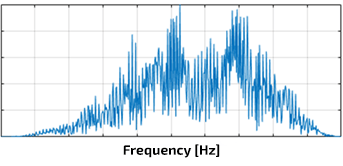
Figure 2. The spectrum of a series of impulse responses

Let’s imagine we have a machine with a damaged bearing that generates impulse responses, but this time the machine is running. Because of that, it generates other numerous components, but as a rule, these components are in a much lower frequency band, i.e. typically from a few Hertz to 2 kHz. These are primarily frequencies coming from the shafts and gears that we mentioned in previous posts. What is worth emphasising, is that they have much more energy than the impulses from the bearings we are looking for.

The envelope analysis consists of removing (filtering out) the signal components in the relatively low band (the result of such an operation in the frequency domain is shown in Figure 2) and finding the answer to the question about the value of the excitation period of the structure (parameter marked in Figure 1). If all vibration signals were easy to analyze, such information could simply be read from the time course, as in synthetic Figure 1. Unfortunately, however, as a rule, bearings in the early stage of damage development generate signals that are orders of magnitude lower than other signal components, therefore impulse responses are not visible on the time waveforms. Figure 3 illustrates this comparison.

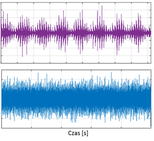
Figure 3. Top: visible damage, bottom: poorly visible damage

One of the most common and effective ways of finding the excitation cycle of a structure, i.e. the next step in envelope analysis, is to construct an entirely new signal whose period expresses the frequency of the pulses, as shown in Figure 4.

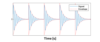
Figure 4. New Signal

Such a signal is constructed by filtering a time signal containing structural vibrations through a low-pass filter. Earlier (for a mathematical reason, which we will omit), we transform the response signal with negative values into positive values (calculate the so-called “absolute value”), i.e. (speaking in the language of electronic engineers) we rectify the signal. Unfortunately, for the data we know nothing about, the selection of the cut-off frequency of the low-pass filter is not obvious, which is why a lot of alternative techniques have been developed over the years. Method

High-pass filter -> absolute value -> low-pass filters

is not the most effective but helps us show the essence of the envelope method.

To illustrate the problem, Figure 5 shows our “new signal” obtained by the low-pass filtration of impulse responses with different values of stop frequency.

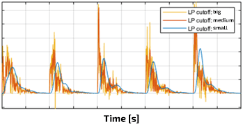
Figure 5. Selection of LP filter parameters in the process of generating envelope signal

In the next part of the analysis, our “new signal” is subjected to the standard procedure of calculating the spectrum, which is called the “envelope spectrum”. An exemplary envelope spectrum is shown in Figure 6:

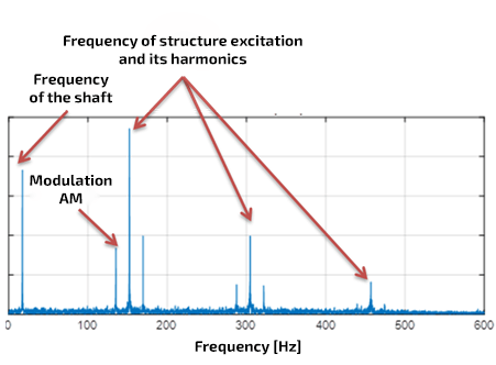
Figure 6. Exemplary envelope spectrum

Looking at Figure 6, one could say that the essence of envelope analysis is that we are not looking for the structural frequencies that are excited, but we are looking for the frequency at which they are excited. Referring to Figure 1, the excitation frequency of structural vibrations, which is one of the so-called “characteristic” frequencies of a bearing is equal to the reciprocal of their excitation period.

How to find the characteristic frequencies of my bearing?

After the introduction, where we showed the methods of signal envelope analysis, let’s go back for a moment to the sentence from the beginning of the post: In the early stage of damage development, the rolling bearing excites its structure and housing according to the so-called “characteristic damage frequency”. Let’s look at the rolling bearing diagram (Figure 7).

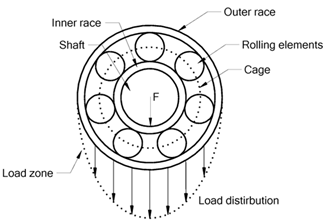
Figure 7. Construction of a rolling bearing (ball bearing)^[2]

Impulse excitation occurs whenever damage appears on any of the cooperating elements. If it is, for example, an Outer Race, then the rolling of each element will cause a miniature strike and the appearance of an impulse. The impulse will excite the structure of the bearing housing and then fade. In a moment, another rolling element will roll over and the situation will repeat itself. Typically, a rolling bearing (because that’s all we’re talking about) can generate several characteristic frequencies, which are listed in Table 1.

Table 1. Characteristic frequencies of a rolling bearing

Acronym	Type of damage	Formula (simplified, 1 race is stationary)
BPFO (Ball Passing Frequency of the Outer Race)	Local damage to the outer race	(nf_r)/2 (1-d/D cosθ)
BPFI (Ball Passing Frequency of the Inner Race)	Local damage to the inner race	(nf_r)/2 (1+d/D cosθ)
BSF (Ball Spin Frequency)	Damage of the rolling element (impact on one of the races)	f_r D/2d [1-(d/D cosθ)^2 ]
FTF (Fundamental Train Frequency) albo Cage	Cage damage	f_r/2 (1-d/D cosθ)

Where:

d – diameter of the rolling element
D –pitch diameter of the bearing(distance between centres of opposite rolling elements)
n – number of rolling elements (in one row)
fr – shaft speed – load angle (typically zero degrees)

Characteristic frequencies can be easily obtained in the VIBnavigator program in the “Kinematics Editor” tab by entering the above data, as shown in Figure 7. These frequencies are also available on the websites of bearing manufacturers.

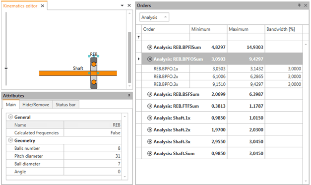
Figure 8. Automatic computing of characteristic frequencies of a bearing

From Figure 8 we can determine, that for example, fundamental frequency BPFO will be tracked in the band 3.05Hz-3.14Hz.

Real-life example

Figure 9 shows the real signal for a bearing in a correct technical condition and a bearing with a damaged inner race. The graphs were made in the VIBnavigator environment, and the data was collected with the AVM 4000 system.

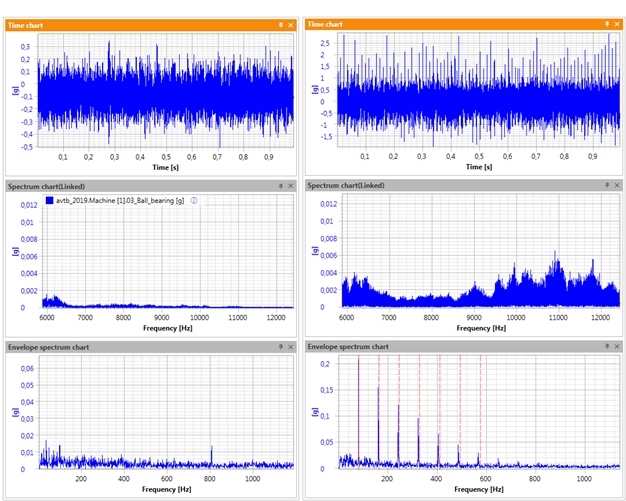
Figure 9. Comparison of bearings: left – good bearing, right – faulty bearing

The upper graphs in Figure 9 show the time courses. Pay attention not only to the characteristic “pins” on the chart but also to the level of value on the horizontal axis – for exemplary significant damage, the increase in value is immense. In the middle graphs, we can see that the damaged bearing induces structural vibrations in the range of 6kHz-12kHz. Finally, on the envelope spectrum (lower graphs), we can practically see measurement noise for the correct bearing, and we can see successive harmonics of the BPFO frequency for the damaged one. Typically, continuous monitoring systems perform bearing failure detection by measuring the PP value and RMS value (see Post #2) of the envelope signal and then identifying the type of failure by tracking the individual characteristic frequencies, e.g. the sum of the BPFOx1, BPFOx2 and BPFOx3 components. There are many materials in the field of bearing diagnostics. We especially recommend the so-called Primers and handbooks from the page ^[3], especially Primer 1982 and Primer 1983 as well as a book ^[4].

Application of measuring equipment

The AMC VIBRO company offers systems that allow detection, identification and assessment of the level of damage to rolling bearings defined automatically on the basis of a kinetostatic model. The user creates the kinematic system of his machine using the simple “drag and drop” method, and the VIBnavigator program calculates all the characteristic frequencies.

	AVM 1000	AVM 2000	AVM 4000
Detection of major bearing damage with the VRMS analysis	✔️	✔️	✔️
Detection of early damage development by tracking spectral bands		✔️	✔️
Detection of early damage development by tracking components of an envelope spectrum		✔️	✔️
Automatic Identification of damage type			✔️
Analysis of envelope spectrum			✔️
Automatic configuration of characteristic frequencies of a bearing			✔️

References

[1] https://doi.org/10.1016/S1350-6307(98)00024-7
[2] Barszcz, Vibration-Based Condition Monitoring of Wind Turbines, Springer 2019
[3] https://www.bksv.com/en/knowledge/library/technical-reviews
[4] R.B. Randall, Vibration‑based Condition Monitoring, John Wiley & Sons, Ltd, 2010
Book recommendation